2. Viewing in graphics - The Orthographic Projection
Now that we've understood all the stages that are involved in the Viewing in graphics. We can move ahead to the meat of this and actually start unravelling the math involved. We will skip the model-matrix transforms that if you don't remember, brings an object from the local/object-space to the global/world-space. As that will be covered in the later sections of this series where we will learn about transforms that move/scale/rotate the objects. For viewing I'm assuming you already know how the translate and scale transform works, as this will be used in the derivation of viewing concepts. I wanted to cover viewing first, I know this is a weird order, but just bear with me!
So, before we can get to the Orthographic Projection we need to understand how a basic Windowing transformation in 2D works. This is nothing but say we have a window - \(w1\) with bottom-left-corner having coordinates \((x_l,y_l)\) and top-right-corner having coordinates \((x_h, y_h)\) & we want to transform it into another window - \(w2\) with bottom-left-corner having coordinates \((x_l',y_l')\) and top-right-corner having coordinates \((x_h',y_h')\). Take a look at Fig-2.1
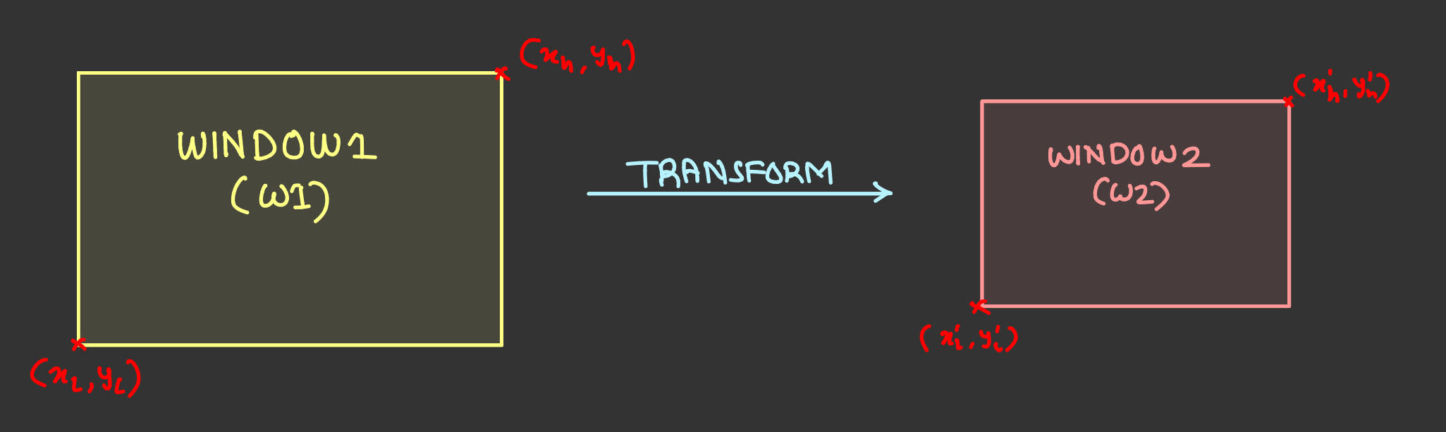
Fig-2.1
Now, that we've defined the problem, we can solve this using 3 simple steps.
1. Step-1: Translating window - \(w1\)'s left-bottom-corner to the orign.
2. Step-2: Scaling window - \(w1\) to the size of window - \(w2\).
3. Step-3: Translating window - \(w1\)'s left-bottom-corner to the position of window - \(w2\)'s left-bottom-corner.
Step-1
To bring the bottom-left-corner of window - \(w1\) to the origin - \((0,0)\), we'll subtract \((x_l,y_l)\) from each of the coordinates of the points of window - \(w1\). This will make the top-right-corner coordinate - \((x_h - x_l, y_h - y_l)\). This can be put up into a 2d-homogenous / \(3 \times 3\) translation matrix as follows:
$$ T_1 = \begin{pmatrix} 1 & 0 & -x_l \\ 0 & 1 & -y_l \\ 0 & 0 & 1 \end{pmatrix} $$
Take a look at Fig-2.2
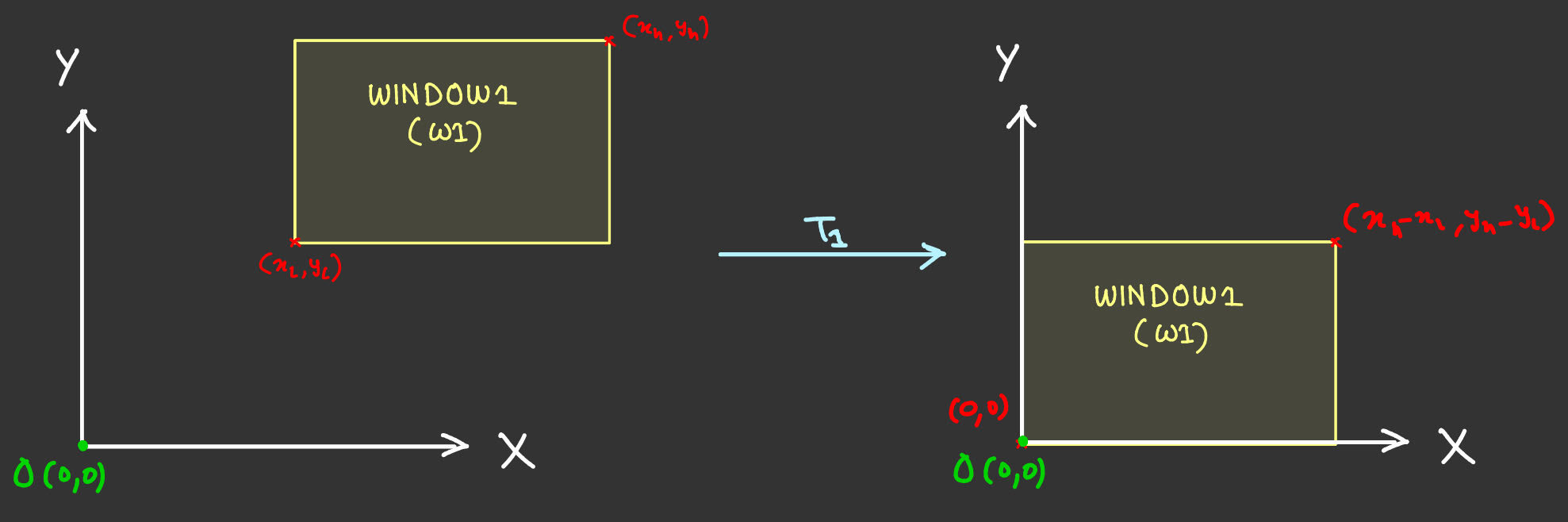
Fig-2.2
Step-2
Now that we've our window-rectangle positioned at the origin (yeah i'll use this phrasing now so that I don't have to say this-bottom-corner all the time lol!). We will now scale it to the size of our desired window - \(w2\) and that can be done in two phases, scaling along \(X\) and \(Y\). We can get the scaling factor by dividing the desired width/height by the current width/height.
For \(X\): \(\frac{x_h' - x_l'}{x_h - x_l}\)
For \(Y\): \(\frac{y_h' - y_l'}{y_h - y_l}\)
This can again be put up into a 2d-homogenous / \(3 \times 3\) scaling matrix as follows:
$$ T_2 = \begin{pmatrix} \frac{x_h' - x_l'}{x_h - x_l} & 0 & 0 \\ 0 & \frac{y_h' - y_l'}{y_h - y_l} & 0 \\ 0 & 0 & 1 \end{pmatrix} $$
Take a look at Fig-2.3
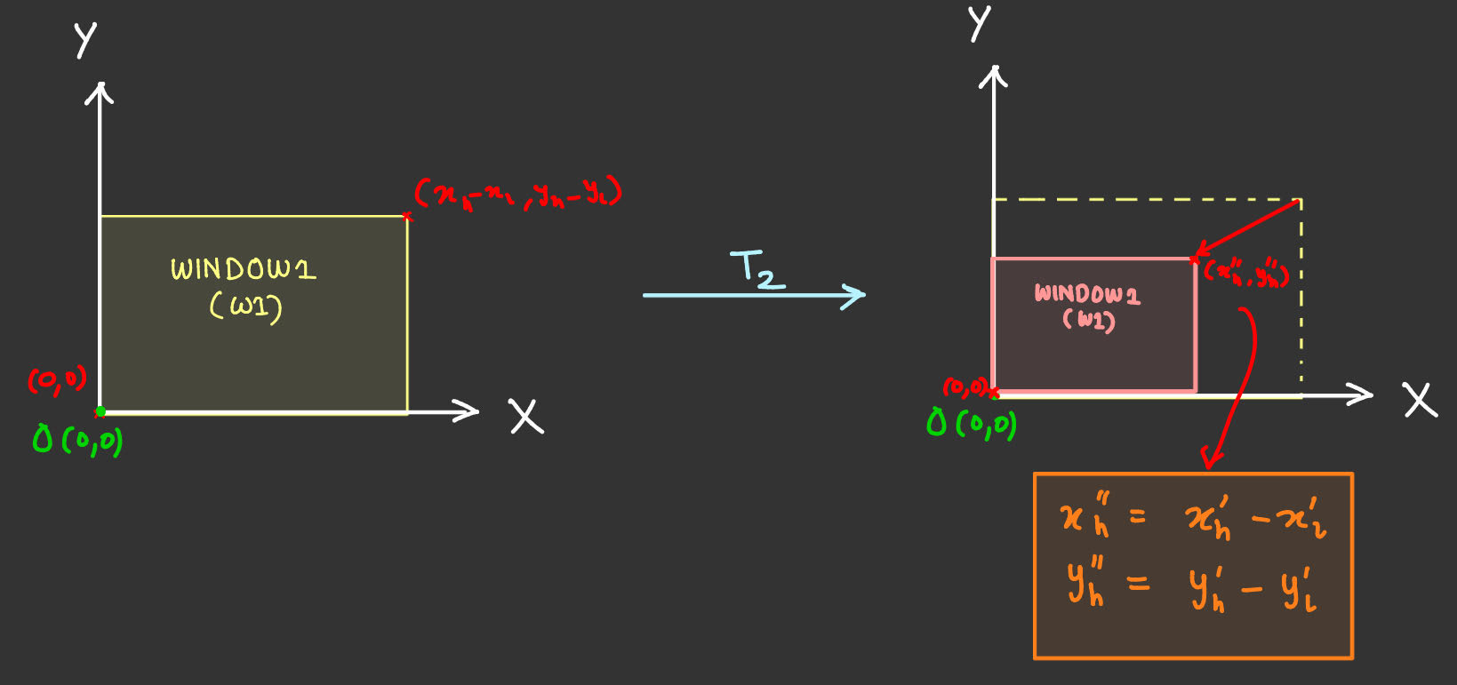
Fig-2.3
Step-3
Finally we just translated our freshly scaled window to the position of window - \(w2\) by adding \((x_l',y_l')\) to each points coordinate of the window-rectangle. This can again be done using a 2d-homogenous / \(3 \times 3\) translation matrix as follows:
$$ T_3 = \begin{pmatrix} 1 & 0 & x_l' \\ 0 & 1 & y_l' \\ 0 & 0 & 1 \end{pmatrix} $$
Take a look at Fig-2.4
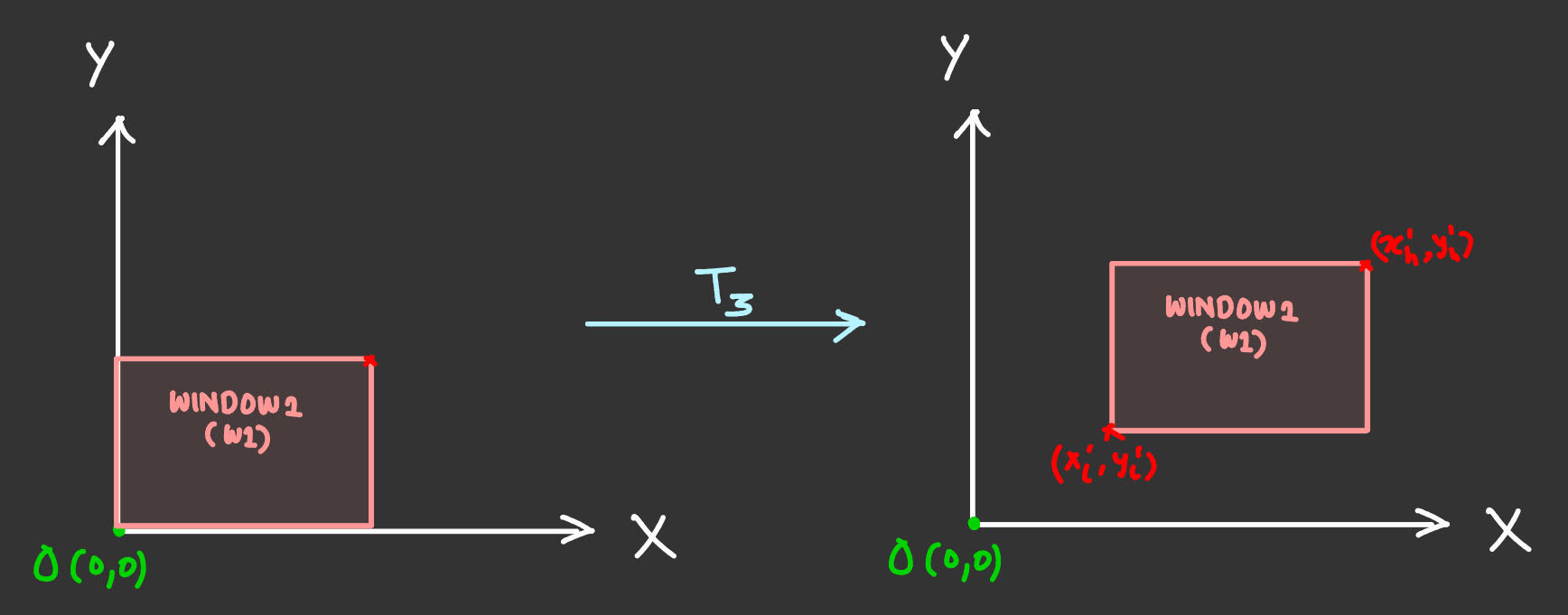
Fig-2.4
Finally we can convert this into a single mapping transformation matrix by chaining all these individual transforms as follows:
$$ T = T_3 \cdot T_2 \cdot T_1 \\ $$
$$ T = \begin{pmatrix} 1 & 0 & x_l' \\ 0 & 1 & y_l \\ 0 & 0 & 1 \end{pmatrix} \cdot \begin{pmatrix} \frac{x_h' - x_l'}{x_h - x_l} & 0 & 0 \\ 0 & \frac{y_h' - y_l'}{y_h - y_l} & 1 \\ 0 & 0 & 1 \end{pmatrix} \cdot \begin{pmatrix} 1 & 0 & -x_l \\ 0 & 1 & -y_l \\ 0 & 0 & 1 \end{pmatrix} $$
Result-2.1: Window transform, rectangle projection
So you might ask, "What does this matrix exactly do?". I've just got the answer for it. It takes the content of the window - \(w1\) and projects them onto window - \(w2\). In simpler terms, it is just like you take out all the things you packed inside a briefcase for a lovely vacation in the Bahamas, you take those packed-items and try to place them in the same position as you placed them into the previous briefcase into a new briefcase of different size. Take a look at the illustration in Fig-2.5
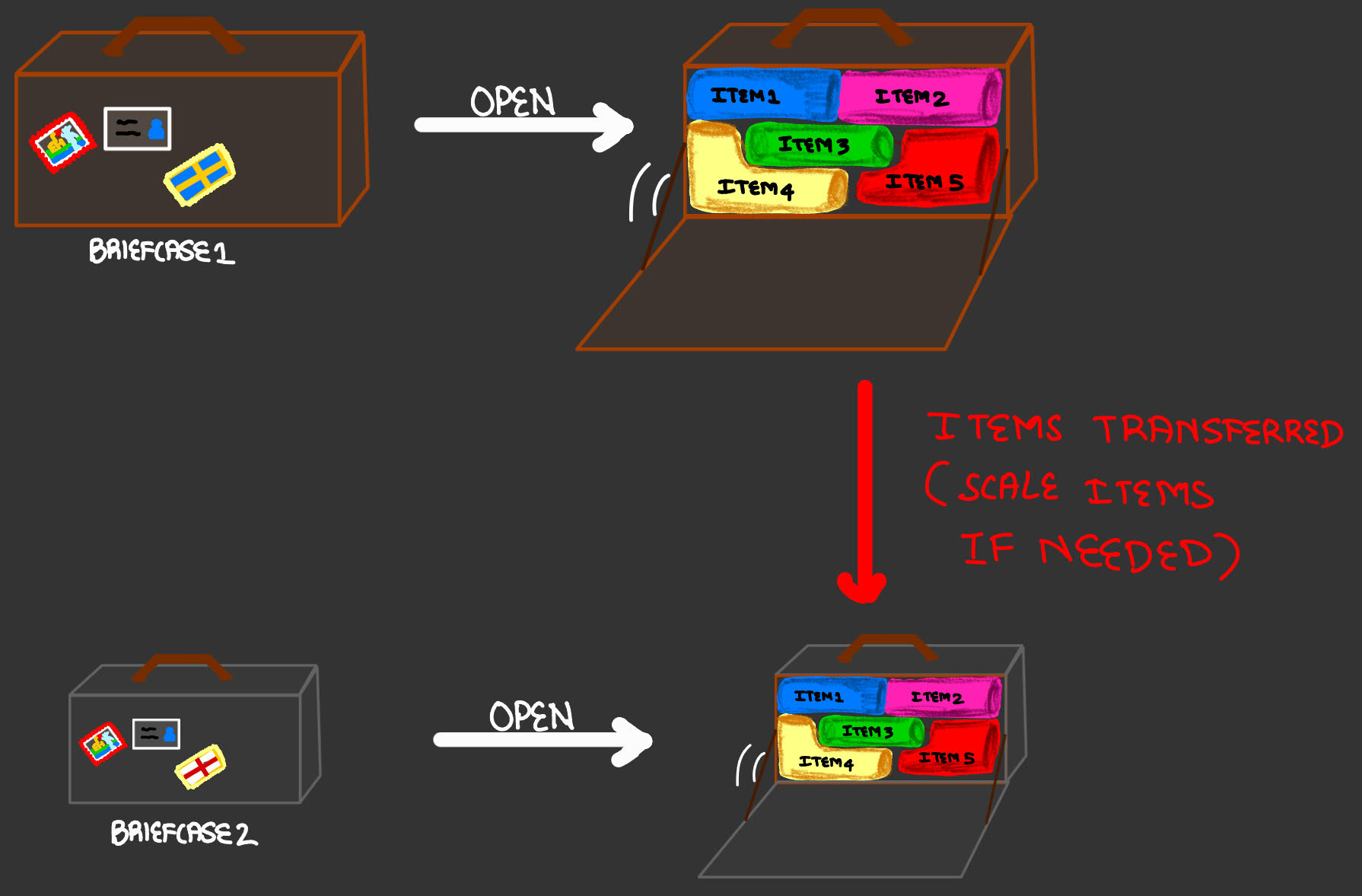
Fig-2.5: Briefcase analogy
Alas! Now you don't have much space to get some goodies from the Bahamas for your girlfriend :(
But, look on the positive sides, folks! We just understood how the window/rectangle mapping works in action with all the depth there is to it. Now We can apply same concept to map or project a cuboid - \(c1\) to a cuboid - \(c2\) by extending it to 3d-homogenous space and using a \(4 \times 4\) transformation matrix as follows:
Result-2.2: 3d cuboid projection
Now, you might ask "How the hell does a cuboid map to another cuboid?", The answer is simple, the rectangular part maps the same as we did before and was well understood with the briefcase analogy. Now, for the third dimension imagine layers of things packed into the briefcase that have to be transferred in the same manner, earlier we scaled along 2 dimensions, now we also squeeze it from top so that all the stuff fits into a more compact briefcase. Watch a pro like Mr. Bean do it, fr... Lol XD.


Fig-2.6: Watch a pro do it in action, projection
Now, that the groundwork is out of our ways. It's time to understand what Orthographic projection truly is. Let's dive deeper into it.
Understanding Orthographic Projection
Orthographic projection is nothing but a parallel projection, we send out parallel rays of ligts and it preserves the actual dimensions of an object. The viewing volume, which is the volume we define. It is nothing but bounds in 3-dimensions till where we can see objects, outside of it objects are not visible or clipped. The viewing volume remains a cuboid in case of orthographic projection. According to the OpenGL conventions, we assume the camera is pointing along \(-Z\)-axis and the view volume is axis-aligned, that is it's faces are parallel to the coordinate axes. We need to define the left, right, bottom, top, near and front bounds for the view volume cuboid. Let's say we set the bounds to \(l, r, b, t, n, f\). Take a look at Fig-2.7 below.
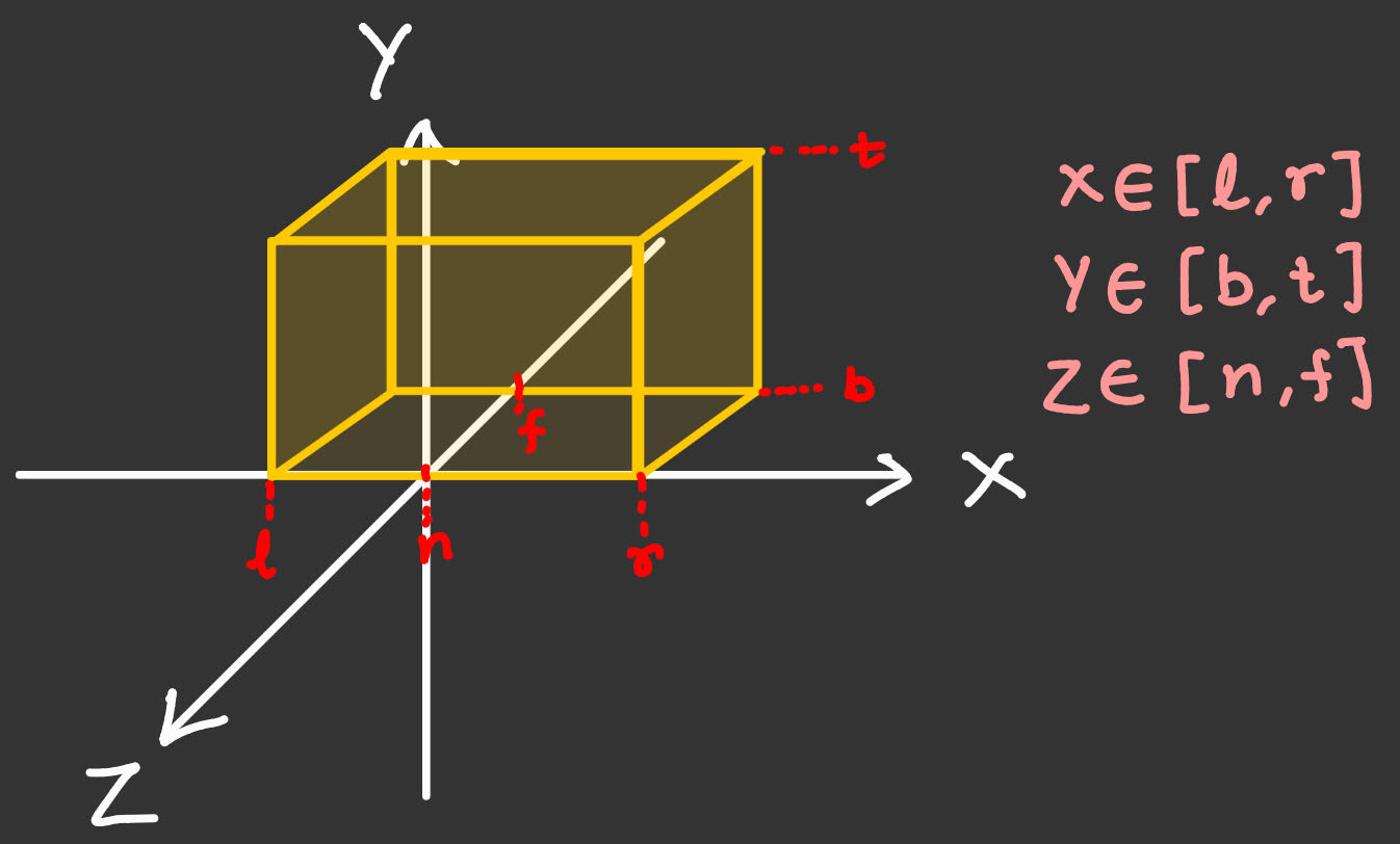
Fig-2.7: View volume for orthographic projection
It is evident from the figure that the cuboid is defined as follows:
\(x \in [l,r] \\ y \in [b,t] \\ z \in [n,f] \)
In orthographic projection, we map/project this cuboid/view-volume we just defined above to something known as the canonical view-volume. Which as discussed in the previous blog is defined as follows:
\(x \in [-1, 1] \\ y \in [-1, 1] \\ z \in [0, 1]\)
It is just as we did when projecting a cube \(c1\) onto another cube \(c2\). And we can directly use that result here and plug in our values, but remember when deriving our result. We had \((x_l, y_l)\) and \((x_h, y_h)\). Similarly here we can see that it is: \((l,b,n)\) and \((r,t,f)\) & \((x_l',y_l')\) and \((x_h',y_h')\) is the coordinates we have to map to, in this case this is the canonical view-volume, so it'll be: \((-1,-1,1)\) and \((1,1,1)\). Let's plug-in these values into the result we derived earlier, into the T-matrix as follows:
$$ T = \begin{pmatrix} \frac{x_h' - x_l'}{x_h - x_l} & 0 & 0 & \frac{x_l' \cdot x_h - x_h' \cdot x_l}{x_h - x_l} \\ 0 & \frac{y_h' - y_l'}{y_h - y_l} & 0 & \frac{y_l' \cdot y_h - y_h' \cdot y_l}{y_h - y_l} \\ 0 & 0 & \frac{z_h' - z_l'}{z_h - z_l} & \frac{z_l' \cdot z_h - z_h' \cdot z_l}{z_h - z_l} \\ 0 & 0 & 0 & 1 \end{pmatrix} $$
Let's call our matrix \(M_{ortho}\) as T sounds too generic :D
$$ T = \begin{pmatrix} \frac{(1) - (-1)}{(r) - (l)} & 0 & 0 & \frac{(-1) \cdot (r) - (1) \cdot (l)}{(r) - (l)} \\ 0 & \frac{(1) - (-1)}{(t) - (b)} & 0 & \frac{(-1) \cdot (t) - (1) \cdot (b)}{(t) - (b)} \\ 0 & 0 & \frac{(1) - (-1)}{(f) - (n)} & \frac{(-1) \cdot (f) - (1) \cdot (n)}{(f) - (n)} \\ 0 & 0 & 0 & 1 \end{pmatrix} $$
$$ M_{ortho} = \begin{pmatrix} \frac{(1) + (1)}{(r) - (l)} & 0 & 0 & -\frac{(r + l)}{(r) - (l)} \\ 0 & \frac{(1) + (1)}{(t) - (b)} & 0 & -\frac{(t + b)}{(t) - (b)} \\ 0 & 0 & \frac{(1) + (1)}{(f) - (n)} & -\frac{(f + n)}{(f) - (n)} \\ 0 & 0 & 0 & 1 \end{pmatrix} $$
Result-2.3: Orthographic projection matrix
Wow, that was a lot! We finally have our orthographic projection matrix, that maps/projects our arbitrary view-volume onto the canonical view-volume. But no projection is complete without being followed by a viewport-transform. It is nothing but projection a 2d axis-aligned rectangle onto another axis-aligned rectangle. Here we want to map this canonical view-volume which is 3d to a viewport/window, a 2d rectangle where we wanna see it. Now this sounds mind-bending right? How can we even project 3d onto 2d?? It's similar to projecting a 2d vector onto a single axis, what we call as breaking a 2d vector into it's 1d components. In simpler terms, imagine our canonical view-volume to be a stack of transparent sheets, which has some drawings on it. Now when you place them on top of each other in the right order based on it's \(z\)-value and observe it from the front, you see a beautiful image, all individual layers coming together to form a single image. Viewport transform is just like that. Take a look at Fig-2.8.
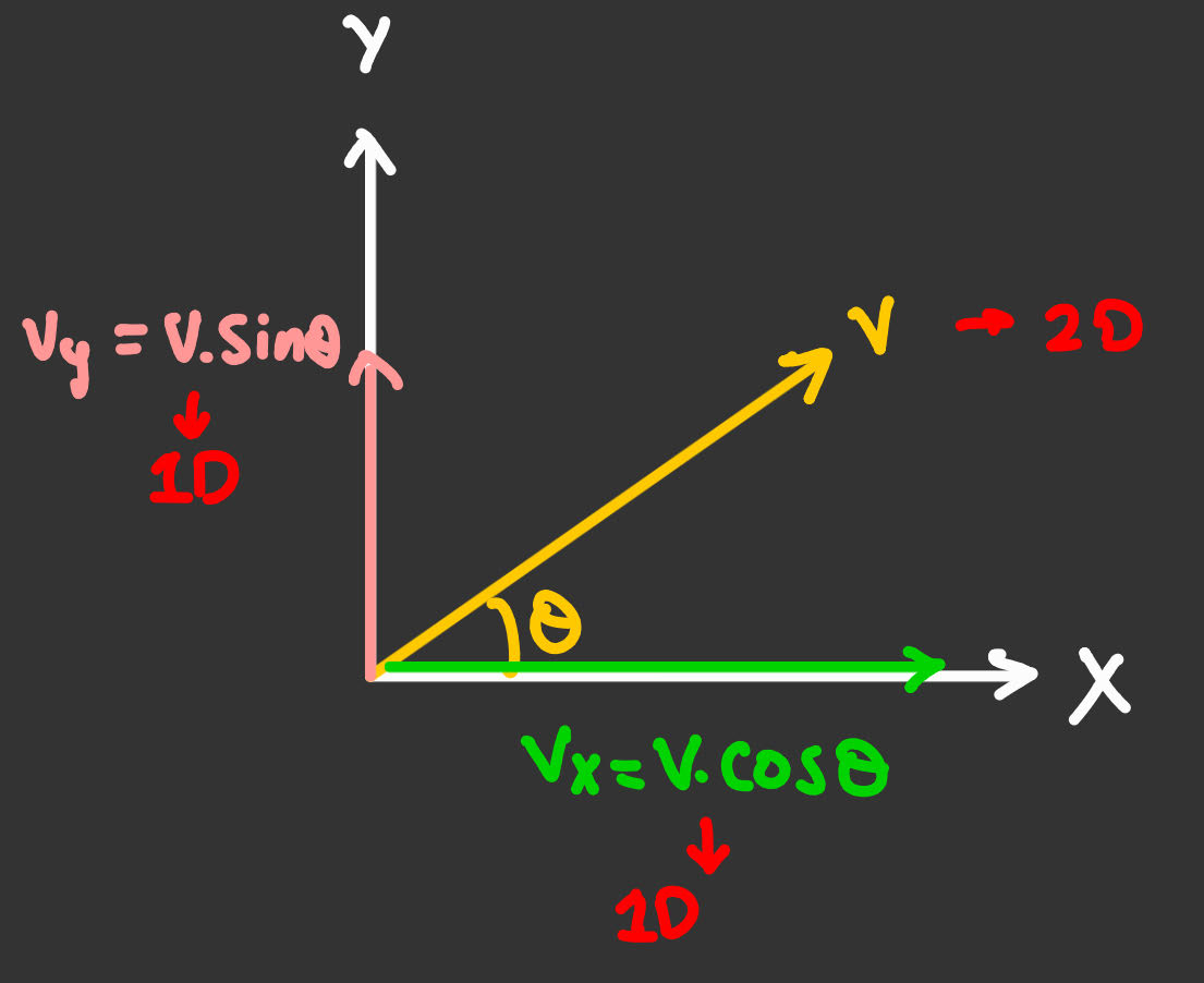
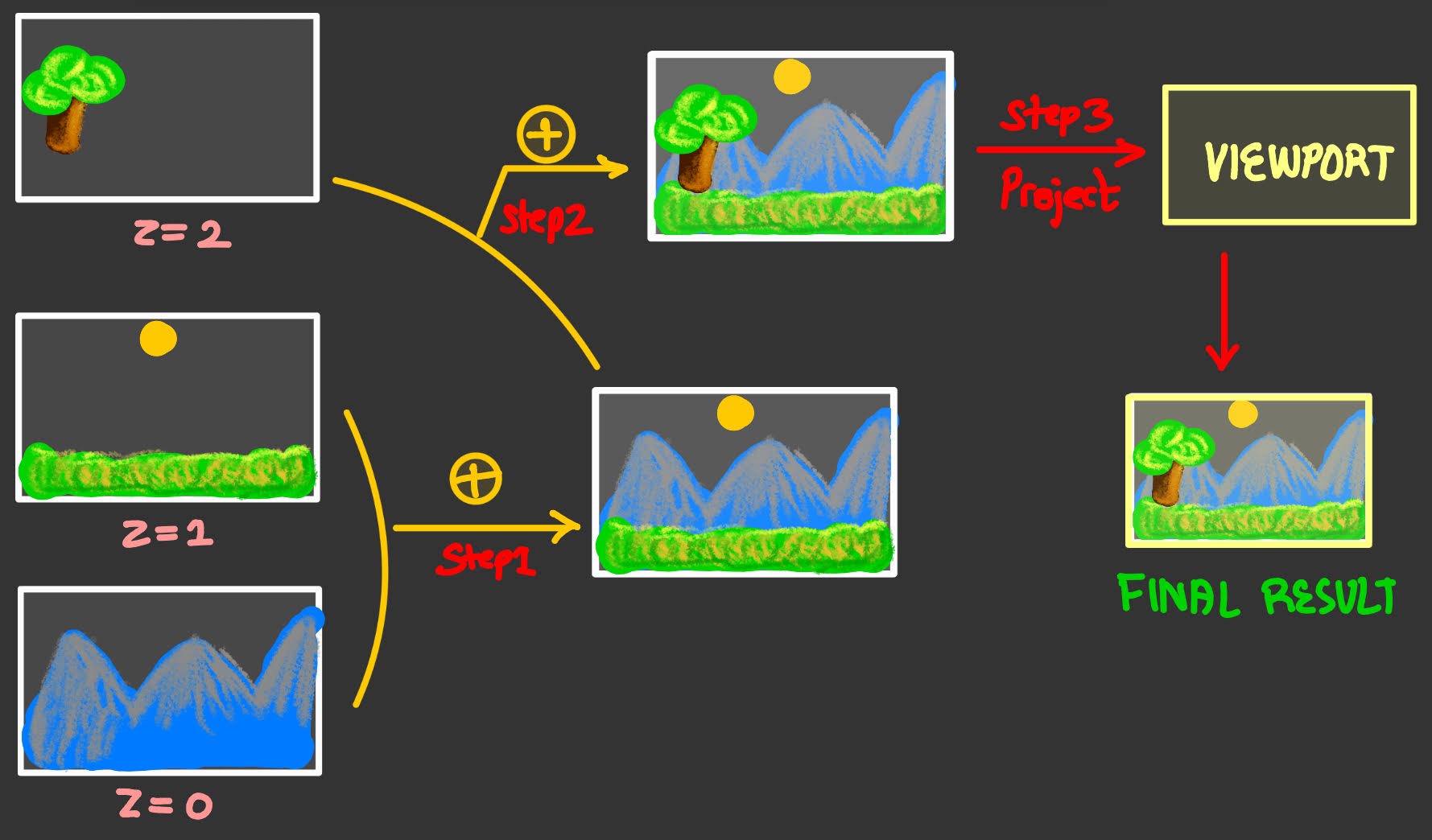
Fig-2.7: Viewport transform analogy, mapping 3d view-volume to 2d rectangle
Now that we've understood this, we can use the window-transform result we obtained at the start and just plug in our values. In this case our \((x_l, y_l)\) will be \((-1,-1)\) and \((x_h, y_h)\) will be \((1,1)\). For the primed-coordinates we'll have to derive one more thing. Let's assume our window/framebuffer is \(n_x\)-pixels wide and \(n_y\)-pixels tall. We have to be a bit clever here, Let's start by understanding a pixel, it's a box and is indexed with it's center and spans \(0.5\)-units on all 4-directions of it's center. So in this case, our \((x_l',y_l')\) wil be \((-0.5, -0.5)\) and \((x_h', y_h')\) will be \((n_x + 0.5, n_y + 0.5)\). Take a look at Fig-2.9 if the derivation is unclear.
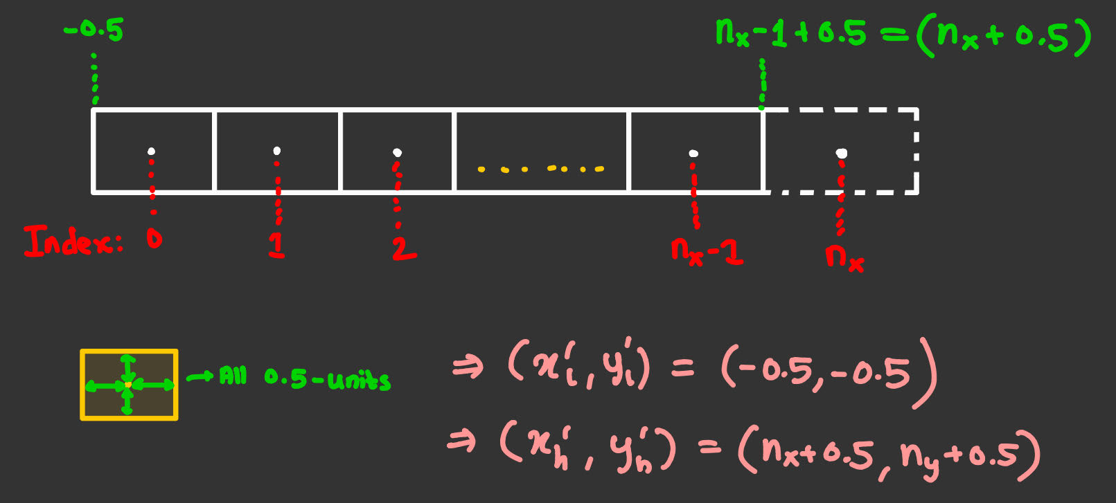
Fig-2.7: Finding the mapping for viewport
Now, let's plug those bad boys into the formula we derived above as follows:
$$ T = \begin{pmatrix} \frac{x_h' - x_l'}{x_h - x_l} & 0 & \frac{x_l' \cdot x_h - x_h' \cdot x_l}{x_h - x_l} \\ 0 & \frac{y_h' - y_l'}{y_h - y_l} & \frac{y_l' \cdot y_h - y_h' \cdot y_l}{y_h - y_l} \\ 0 & 0 & 1 \end{pmatrix} $$
$$ T = \begin{pmatrix} \frac{(n_x + 0.5) - (-0.5)}{(1) - (-1)} & 0 & \frac{(-0.5) \cdot (1) - (n_x + 0.5) \cdot (-1)}{(1) - (-1)} \\ 0 & \frac{(n_y + 0.5) - (-0.5)}{(1) - (-1)} & \frac{(-0.5) \cdot (1) - (n_y + 0.5) \cdot (-1)}{(1) - (-1)} \\ 0 & 0 & 1 \end{pmatrix} $$
$$ T = \begin{pmatrix} \frac{n_x}{2} & 0 & \frac{n_x - 1}{2} \\ 0 & \frac{n_y}{2} & \frac{n_y - 1}{2} \\ 0 & 0 & 1 \end{pmatrix} $$
But, this is for 2d, we need to consider \(z\)-axis aswell, although we don't change it but we want it for the depth information later when we wanna do depth-testing so to keep it we add a row and column to carry the z-coordinate without changing it as follows:
Result-2.4: Viewport projection matrix
And we call it the \(M_{vp}\) matrix. And finally we are ready to perform orthographic projection on any 4d vector in 3d-homogenous space. We first apply the \(M_{ortho}\) matrix to it, followed by the \(M_{vp}\) matrix to present our object onto the screen, under orthographic projection. Do note that we are using the column-major format and we multiply these transformation matriceson the left of the vector and they are applied in the right-to-left order.
$$ \begin{pmatrix} x_{pixel} \\ y_{pixel} \\ z_{canonical} \\ 1 \end{pmatrix} = (M_{vp} \cdot M_{ortho}) \cdot \begin{pmatrix} x \\ y \\ z \\ 1 \end{pmatrix} $$
Now doing all that jazz, we get the exact integer-coordinates \((x_{pixel},y_{pixel})\) with which we can just index into the framebuffer for a particular pixel and we get \(z_{ndc} or z_{canonical}\) which is just the normalized \(z-coordinate \in [-1,1]\) and later after rasterization we can perform depth-testing and for that we've to map this \(z-coordinate -> [0,1]\), which can be achieved by this formula \(\frac{1 + z_{ndc}}{2}\)
Voila! We've successfully understood the math behind doing orthographic projection and viewport transformation. If you have made it till here, you are definitely a courageous one! That was a lot to grasp. But most of our groundwork is laid here and in later continuations of this blog, I'll be referring to results from here and it'll be much shorter I promise. Peace! :D
NEXT-BLOG: 3. Viewing in graphics - The Camera Transformation