3. Viewing in graphics - The Camera Transformation
"Well, well... Look, who do we have here?" Aren't you tired already from the last blog? I mean it was kind of a math monster, won't you agree? Compared to the last-blog this is going to be a cake walk. Yeah, trust me... See it for yourself. But yeah this topic is quite important, The camera transformation allows to see the world through the lens of a sweet-little virtual-camera. This will give you the ability to attach this camera to your game-character and follow it and do a lot's of cool stuff. Like you can attach this camera to a FPS-hands model and baammmm! you've made yourself a simple fps setup, and now you can make the camera move based on inputs from keyboard for walking and looking around with mouse movements. I hope this hypes you up for what comes next.... Tons of Math! Lol..

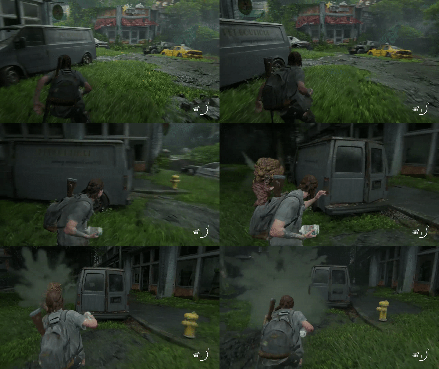
Fig-3.1: Yeah! you can create such fps/tps-setup after learning this, you'll surely be able to build a character controller.
Now, let's start by understanding what a virtual-camera is in the first place. It is as its name suggests, a camera that we define in code (simply mathematical-transformations) and do not mistake it by any floating object in our game world... NO! (большое нет), we apply this so-called virtual-camera transform to each and everything we render in our virtual-world and this transforms or changes objects positions as seen through the lens of our virtual-camera. Before we define our virtual-camera using the mathematical-construct, let's undestand how basis-transformation works and what is it exactly, as this is the meat of our camera-transformation.
Basis vectors are orthonormal vectors, meaning that they are normalized(having magnitude = 1) and are mutually-perpendicular to each-other. Just like the Canonical Basis, - \(\{x,y,z\}\) which are mutually-perpendicular to each other and all have a unit magnitude. These basis are represented as vectors as follows:
$$ x = \begin{pmatrix} 1 \\ 0 \\ 0 \end{pmatrix} \; y = \begin{pmatrix} 0 \\ 1 \\ 0 \end{pmatrix} \; z = \begin{pmatrix} 0 \\ 0 \\ 1 \end{pmatrix} $$
Any coordinate-system/frame is defined by a point \(P\)(origin) and \(\{u,v,w\}\) its basis vectors. Our Canonical Frame is defined by the origin \(O=(0,0,0)\) and the basis vectors \(\{x,y,z\}\). Now that we understand what a coordinate-system/frame is, we can move forward and understand the change of basis through an example.
Case1: Say we have a car-racing game and the player sees the world in a first-person view, that is they see the world through the windshield of the car. Now we do a trick when the car moves, we keep the car's dashboard and everything as a static overlay, drawn on top of the world which just moves in the opposite direction. Here, we can safely say that the coordinate-system/frame or our frame-of-reference is the car and the world moves with-respect-to this car/frame-of-reference.
Case2: Another way to see this is, say our racing game is now in third-person view and we see the car from a camera floating above it. Now it makes sense to keep the world static and move the car around with-respect-to the frame-of-reference, which is the world-origin. Take a look at Fig-3.2 for a better understanding.

Case1

Case2
Fig-3.2
The point of this analogy was to explain the fact that any point in the world can be defined with-respect-to different frame-of-references. For example, your favourite pizza place might be 200m away from your place, but might be miles away from mine. See, all depends on the frame-of-reference, who's the observer, the observer decides it all. Take a look at Fig-3.3 for a better understanding.
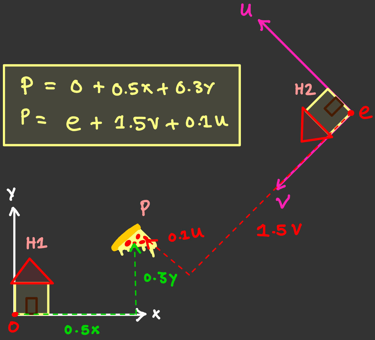
Fig-3.3: Frame of reference
But, say that you wanna invite your girlfriend to the same pizza place for a date. Now you've to communicate the location of this pizza place to her using a frame-of-reference that she understands. You can't tell her that this place is \(0.5 \cdot x + 0.3 \cdot y\) from my place, you need to tell her the location from her home's frame-of-reference so that she can make it to the date. Telling her the location from her frame-of-reference is what we call as Basis/Frame Transformation. Note that we are using these terms loosely, basis transformation is actually related when we change the basis-vectors but keep the origin fixed, and frame-transformation involves change of basis-vectors and also the origin. So, for this blog we will use these terms to mean the same. "Mathematicians are gonna kill me for sure! Lol.."
This basis-transformation is nothing but expressing one set of basis vectors in terms of other. That's it, its that simple. Let's understand the math behind this from Fig-3.3, it can be done in two easy steps as follows:
Step1:
We first translate the origin of your frame-of-reference to the origin of her frame-of-reference (the Canonical frame-of-reference). We can achieve this by creating a translation matrix as follows:
Result-3.1: Translation matrix to translate your frame-of-reference's origin to hers
Take a look at Fig-3.4 for a better understanding.
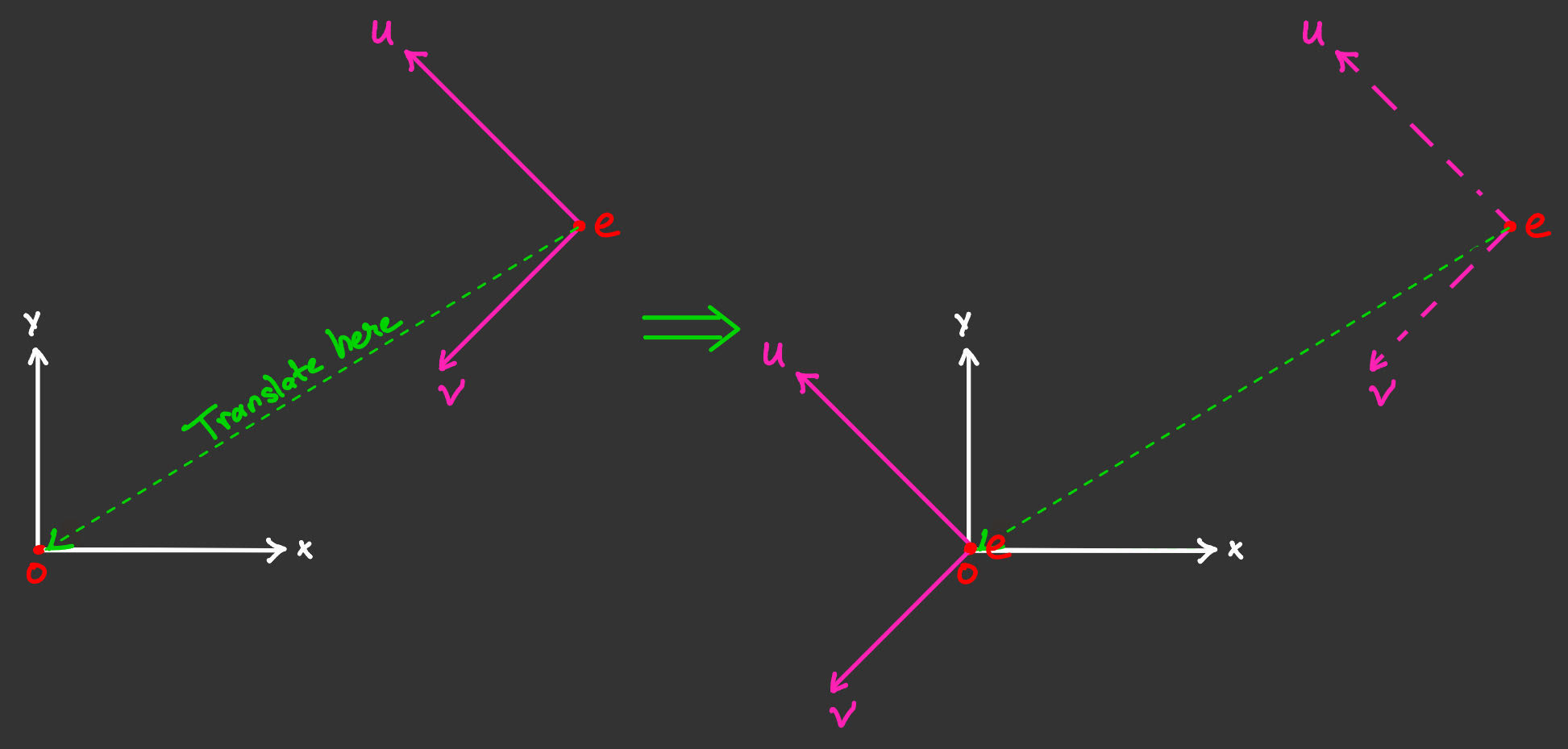
Fig-3.4: basis-transformation - translation
Step2:
We then rotate your frame-of-reference to match the orientation of her frame-of-reference (the Canonical frame-of-reference). We can achieve this by creating a rotation matrix as follows:
Result-3.2: Rotation matrix to rotate your frame-of-reference to hers
We're again using the column major format, and the first column corresponds to the basis vector \(u\) and the second corresponds to \(v\). Also, \(u_x\) means component/projection of vector \(u\) along \(x\), we've just written each in terms of the basis \(\{x,y\}\), this will rotate your frame-of-reference to hers. Take a look at Fig-3.5 for a better understanding.
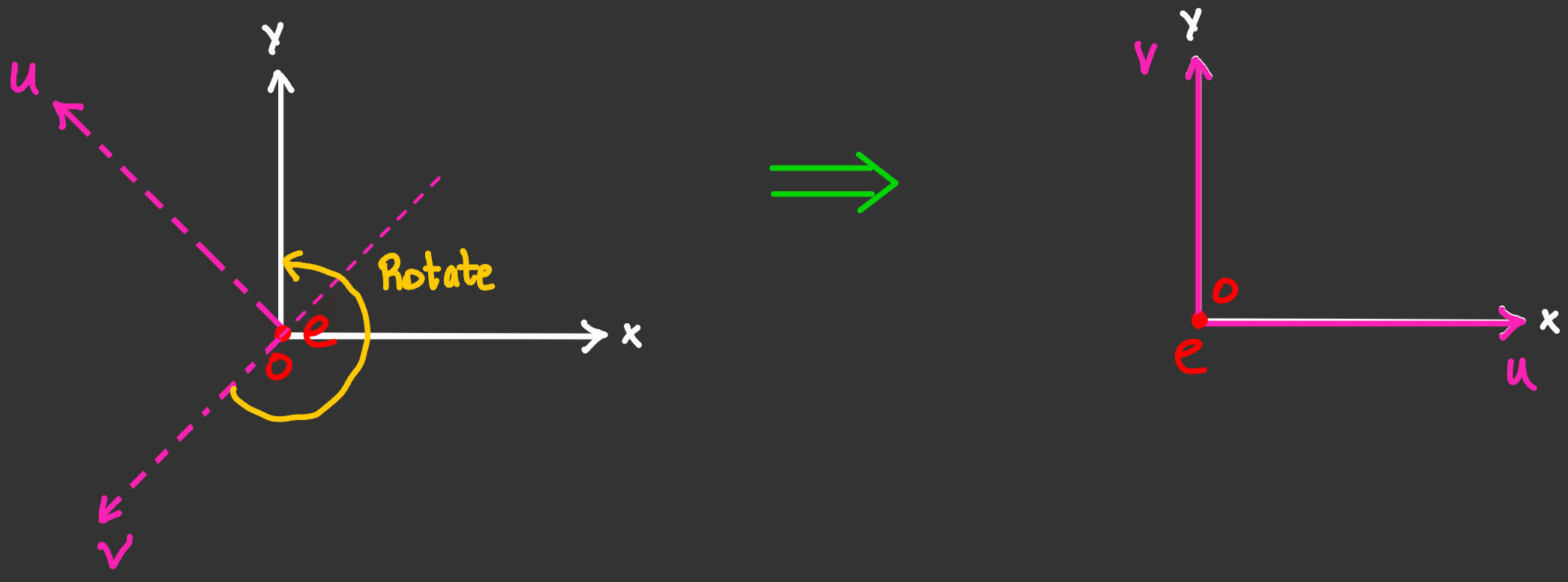
Fig-3.5: basis-transformation - rotation
Now let's accumulate both of the transforms into a single matrix, note that these are in column-major format, so the transforms are applied from right to left as follows:
$$ M = R_{2d} \cdot T_{2d} $$
$$ M = \begin{pmatrix} x_u & x_v & 0 \\ y_u & y_v & 0 \\ 0 & 0 & 0 \end{pmatrix} \cdot \begin{pmatrix} 1 & 0 & x_e \\ 0 & 1 & y_e \\ 0 & 0 & 1 \end{pmatrix} $$
$$ M = \begin{pmatrix} | & | & | \\ u & v & e \\ | & | & | \\ 0 & 0 & 1 \end{pmatrix} $$
Now, if we apply this transformation to the vector associated with the pizza place, defined with with-respect-to your frame-of-reference \(v_p\). It will transform \(v_p\) to \(v_p'\), which is just the same place, but with-respect-to your girlfriend's frame-of-reference.
But in our case we're more interested in bringing a vector defined in the canonical-frame to our specified frame, which is the camera-frame. Connecting this to the analogy of pizza place and girlfriend. Given any vector \(v_p'\) to the pizza place with-respect-to your girlfriend's frame-of-reference, we want to find \(v_p\) which is in your frame-of-reference. In short, our basis-change matrix is basically the inverse of what we had before \(M_{basis-change} = M^{-1}\)
$$ M_{basis-change} = \begin{pmatrix} | & | & | \\ u & v & e \\ | & | & | \\ 0 & 0 & 1 \end{pmatrix} ^{-1} $$
This can be extended to 3-dimensions as follows:
Result-3.3: Matrix for basis-change
Now, that we've understood the math behind basis-change we can finally understand the camera-transformation. Let's define our virtual-camera first. Let's say that our camera is located at the origin \(e\) and has the basis \(\{u,v,w\}\) and let's say we've additional two vectors. Gaze - where our camera looks \(g\) and top - which points to the top of our view-volume \(t\). Take a look at Fig-3.6 for a better understanding.
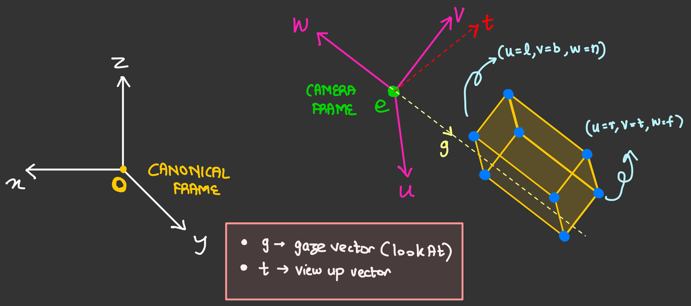
Fig-3.6: Virtual camera setting
Now, we understand the setting of our virtual-camera and the gaze vector \(g\) and top vector \(t\) is already known in terms of canonical basis and \(e\) is already in canonical basis as it is the camera position that we define in canonical basis. Now the only thing that is left to find the camera-basis \(\{u,v,w\}\) in terms of the gaze vector \(g\) and top vector \(t\) and the camera position \(e\). This can be done as follows:
basis vector \(w\) can be written as negative of \(g\) as seen in Fig-3.6
Result-3.4
For the basis we require normalized vectors, and so we divide \(g\) by its norm or magnitude represented by the notation \(||g||\).
Now we can get the right-vector \(u\) by taking a cross-product between \(t\) and \(w\) which is quite evident from Fig-3.6.
Result-3.5
Now that we've two of the three basis vector the third one \(v\) can be found by taking the cross-product of the two we know.
Result-3.6
Now that we've found the basis for camera in terms of our canonical basis. We just plug these into Result-3.3 and we have our camera transform.
$$ M_{basis-change} = \begin{pmatrix} | & | & | & | \\ u & v & w & e \\ | & | & | & | \\ 0 & 0 & 0 & 1 \end{pmatrix} ^{-1} $$
This can be expanded as follows:
$$ M_{basis-change} = \begin{pmatrix} \begin{pmatrix} u_x & v_x & w_x & 0 \\ u_y & v_y & w_y & 0 \\ u_z & v_z & w_z & 0 \\ 0 & 0 & 0 & 1 \end{pmatrix} \cdot \begin{pmatrix} 1 & 0 & 0 & x_e \\ 0 & 1 & 0 & y_e \\ 0 & 0 & 1 & z_e \\ 0 & 0 & 0 & 1 \end{pmatrix} \end{pmatrix} ^ {-1} $$
Now we can make use of the inverse-property of matrices: \((A \cdot B)^{-1} = B^{-1} \cdot A^{-1}\)
$$ M_{basis-change} = \begin{pmatrix} 1 & 0 & 0 & x_e \\ 0 & 1 & 0 & y_e \\ 0 & 0 & 1 & z_e \\ 0 & 0 & 0 & 1 \end{pmatrix}^{-1} \cdot \begin{pmatrix} u_x & v_x & w_x & 0 \\ u_y & v_y & w_y & 0 \\ u_z & v_z & w_z & 0 \\ 0 & 0 & 0 & 1 \end{pmatrix}^{-1} $$
Now the inverse of the translation part will just flip the signs and for the rotation part we've to find the inverse for-real. But don't worry, "Matrix property comes to our rescue!". It is known that inverse of a orthonormal square-matrix is equivalent to its transpose. Let's apply that.
$$ M_{basis-change} = \begin{pmatrix} 1 & 0 & 0 & -x_e \\ 0 & 1 & 0 & -y_e \\ 0 & 0 & 1 & -z_e \\ 0 & 0 & 0 & 1 \end{pmatrix} \cdot \begin{pmatrix} u_x & v_x & w_x & 0 \\ u_y & v_y & w_y & 0 \\ u_z & v_z & w_z & 0 \\ 0 & 0 & 0 & 1 \end{pmatrix}^{T} $$
$$ M_{basis-change} = \begin{pmatrix} 1 & 0 & 0 & -x_e \\ 0 & 1 & 0 & -y_e \\ 0 & 0 & 1 & -z_e \\ 0 & 0 & 0 & 1 \end{pmatrix} \cdot \begin{pmatrix} u_x & u_y & u_z & 0 \\ v_x & v_y & v_z & 0 \\ w_x & w_y & w_z & 0 \\ 0 & 0 & 0 & 1 \end{pmatrix} $$
$$ M_{basis-change} = \begin{pmatrix} u_x & u_y & u_z & -x_e \\ v_x & v_y & v_z & -y_e \\ w_x & w_y & w_z & -z_e \\ 0 & 0 & 0 & 1 \end{pmatrix} $$
We change \(e\)'s coordinates with-respect-to our camera-frame, by taking dot-product with each of the basis vectors of our camera. As the translation must happen with with-respect-to the camera
$$ M_{basis-change} = \begin{pmatrix} u_x & u_y & u_z & -(u \cdot e) \\ v_x & v_y & v_z & -(v \cdot e) \\ w_x & w_y & w_z & -(w \cdot e) \\ 0 & 0 & 0 & 1 \end{pmatrix} $$
let's call this matrix \(M_{cam}\) and using Result-3.4, Result-3.5, Result-3.6, we get:
Result-3.7: Camera transformation matrix
We have finally derived the camera transformation matrix. Now you just need to update this matrix every frame based on player-position and the look-at vector and you have yourself a character controller setup. And you can use it in the following way, given that you already have the \(M_{ortho}\) ready with you:
$$ \begin{pmatrix} x_{pixel} \\ y_{pixel} \\ z_{canonical} \\ 1 \end{pmatrix} = ( M_{vp} \cdot M_{ortho} \cdot M_{cam}) \cdot \begin{pmatrix} x \\ y \\ z \\ 1 \end{pmatrix} $$
Wooohoooo! Give yourselves a good pat on your back and treat yourself with a cup of coffee and your favourite snack. We just have one more blog to go, in which we will learn about perspective projection and then we are done with viewing in graphics.

NEXT-BLOG: 4. Viewing in graphics - The Perspective Projection